Introduction
Goldman Sachs has a private cloud spanning data centers around the world. These data centers house a large number of cooperating hardware and software components, such as hosts, storage devices, network links, databases, message queues, caches, load balancers, etc. All of these components have finite capacity, and the exhaustion of this capacity could impact the resilience of necessary applications. Furthermore, in some cases, provisioning additional capacity can require some time, and hence it cannot be performed reactively in real-time (that is, immediately post exhaustion). Ideally, any approach to guarantee the availability of sufficient capacity must be proactive.
Viable approaches must also be sufficiently accurate, so as to not overwhelm users with notifications or lead to costly over-provisioning of resources, while not missing any potential capacity exhaustion scenarios. Such approaches must also be designed to handle the vagaries in resource utilization and be able to distill the signal from the noise.
In this blog post, we will explore a novel machine learning-based forecasting pipeline that uses a diverse array of techniques, including a patent pending change point detection algorithm to predict capacity outages ahead of time, thereby enabling infrastructure owners to take preventive action. Additionally, we also discuss how we apply the same forecasting approach to detect whether the real-time utilization of these components is anomalous and requires immediate attention. Such situations of anomalous behavior largely arise when the utilization surges significantly which results in bringing the component to the verge of exhaustion. In these cases, our system raises real-time alerts that notify owners about the anomalous behavior, thereby enabling them to temporarily mitigate the issue(s) while longer-term solutions are planned.
The Capacity Planning Problem Statement
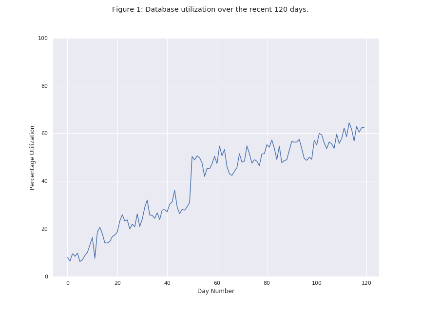
In order to explain the approach we took when building the system, we will use the following problem statement: Given the past space utilization for a database (example - figure 1), predict when its space utilization is likely to hit 100%. This information can be used to trigger alarms early and give database administrators enough time to mitigate the issue by provisioning additional capacity, reducing consumption through archiving, and so on.
A Brief Overview of Our Approach
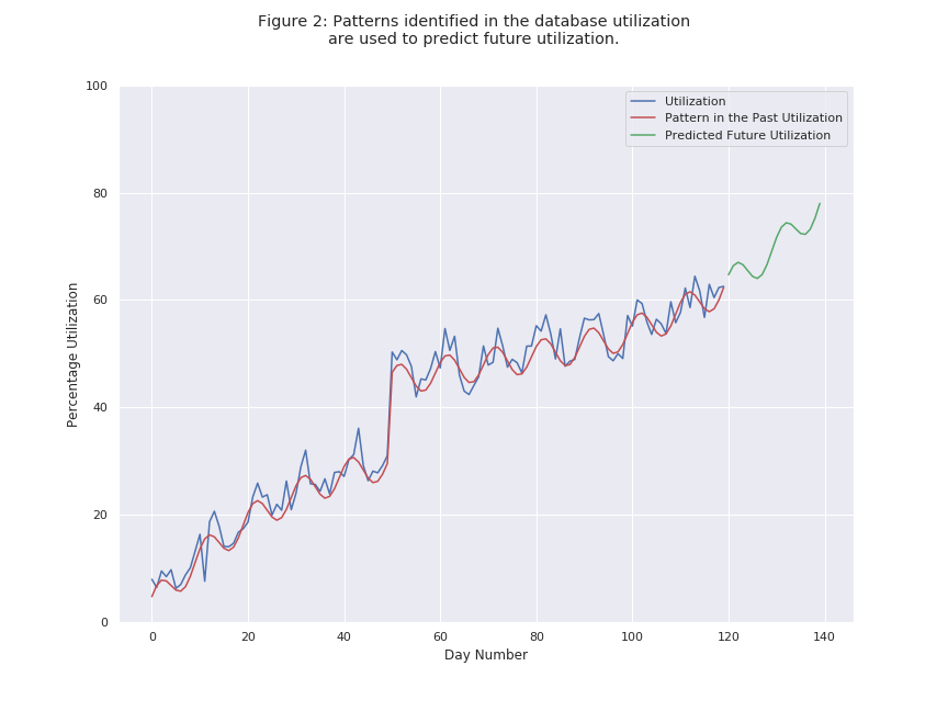
This problem statement is a classic, well-studied machine learning problem called time series forecasting. A time series captures the variation of a metric over time. For our problem, the metric would be the database space utilization, and the time series would describe its variation over a long period of time. Time series forecasting is the problem of making predictions about the future values of a metric by identifying patterns present in its past behavior. For example, for the time series in Figure 2, we identify a steady upward growth demarcated by the red line in the below image (more on this below). We use this upward growth pattern to make predictions into the future - represented by the green line in Figure 2.
In other words, the green line represents an approximate estimate for the utilization of this database in the near future, and this estimate can then be used to predict the future date of a potential capacity outage. This prediction is the valuable information that time series forecasting provides.
As with most machine learning problems, our approach towards a solution began with the exploration of a large dataset of past utilization time series for various kinds of infrastructure components. We looked for various kinds of patterns that might exist (such as the steady upward growth that we just discussed). For each of these patterns, we researched and narrowed down the appropriate machine learning techniques to maximize the accuracy of our prediction. Finally, after numerous rounds of backtesting and validation with these techniques, we built a system that makes high-quality forecasts for infrastructure utilization.
Patterns Identified
Some of the fundamental time series patterns that we identified during data exploration are listed in Table 1. Any time series we encounter can be a combination of one or more such fundamental patterns. Moreover, each of the patterns presents its own challenge, and needs distinct machine learning techniques to model. In this blog post, we will cover only some of the modeling techniques.
.png)
Figure 3(a): Pattern = Trend; Definition = Continuous growth / reduction in utilization.
.png)
Figure 3(b): Pattern = Change point; Definition = Sudden shift in utilization in short spans of time.
.png)
Figure 3(c): Pattern = Seasonality; Definition = Periodic patterns in utilization over time.
Machine Learning System Architecture
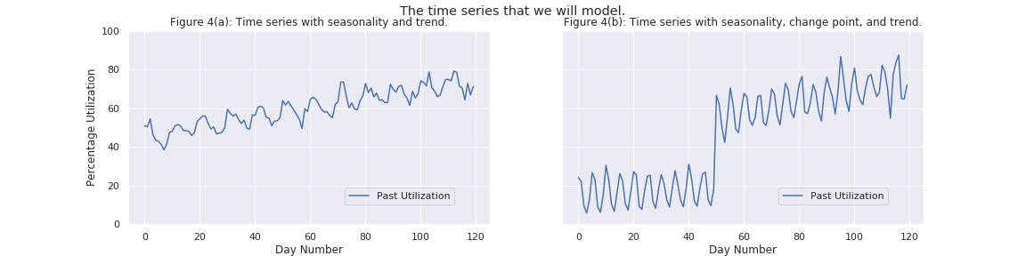
We will use the two time series in Figure 4 to explain the step-by-step architecture of the machine learning system. The time series in Figure 4(a) has seasonality (a repeating component) and a trend, while the time series in Figure 4(b) has seasonality, a trend, and a change point (sharp jump) around Day Number 50.
Extracting a Seasonal Component
To begin, the model extracts the seasonal component (a periodic pattern of the kind displayed in Figure 3(c)) from these time series in Figure 4. This breaks down the overall time series into two pieces - the part of the time series that repeats periodically and whatever is left over. This is highlighted in Figure 5, where the top plot shows the percentage utilization for a disk, the middle shows its extracted seasonal component, and the bottom shows the leftover component.
Note that when we sum up the two components - the middle seasonal component and the bottom leftover component, we will get the top overall time series. That is,
Overall time series (Top) = A Seasonal Component (Middle) + A Leftover Component (Bottom)
In order to extract the middle seasonal component (the one that periodically repeats), we use a couple of well-studied machine learning techniques known as Seasonal-Trend Decomposition (more info here, here, and here) and Periodogram Estimation (more info here and here).
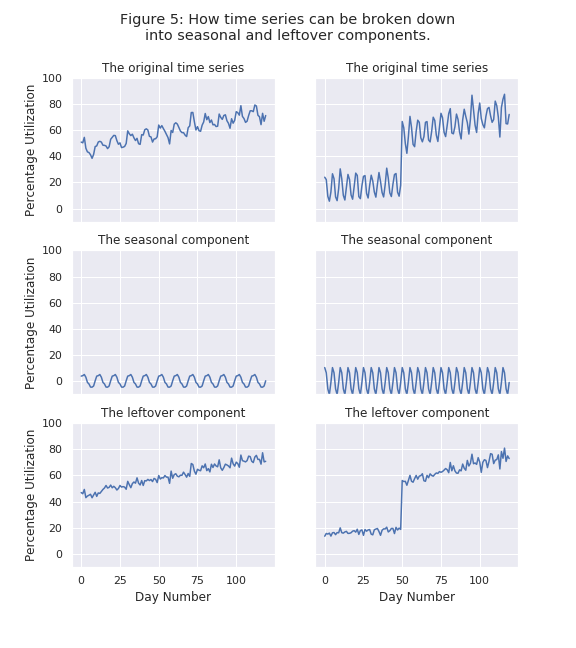
The reason we break down these time series into seasonal and leftover components is because it simplifies our machine learning problem. There are a number of well-studied machine learning techniques to build models for purely seasonal time series and for time series that have no seasonality in them. By breaking our time series down in this manner, we can filter the noise (in this case, the repeating, predictable seasonal component) from the useful data (the anomalies in the leftover component).
Detecting Change Points
Once the seasonal component has been extracted, we then take the leftover time series and run a proprietary algorithm that we have developed to identify the time of the change point (a sharp jump) in the time series, if any. This algorithm is a modification of the well-known CUSUM change point detection algorithm, and further details about it can be found in our patent. Our algorithms are capable of detecting change points in the presence of an underlying trend. The results of this algorithm are shown in Figure 6 - no change point was detected in the image on the left while a change point was indeed detected on the image on the right on Day Number 50.
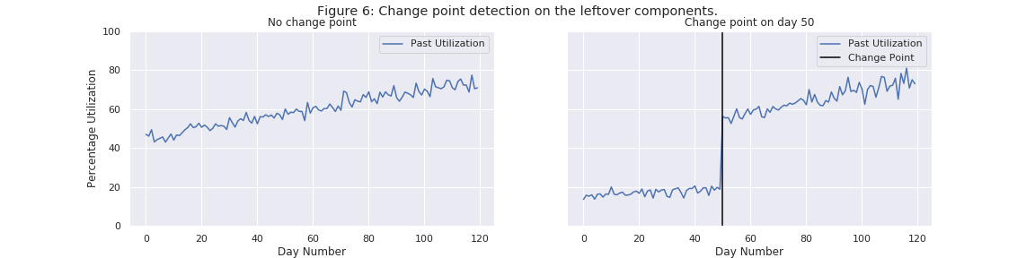
Again, the rationale for detecting change points is so that our model can work around them - there exist well-studied techniques to model time series without change points or seasonal patterns which can now be used out-of-the-box.
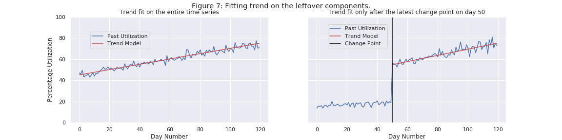
Fitting Trends
Finally, once we know whether there is a change point and, if so, where, then we can fit the trend using a classic machine learning technique known as ridge regression (more info here and here). When we fit the ridge regression model (or any machine learning model in general), it gives us a mathematical rule that describes the underlying pattern in the data. In Figure 7, the pattern identified by the mathematical rule is highlighted in red. Additionally, when there exist change points in the time series, we fit our trend model only to the portion after the latest change point. This is because a change point is a place where the behavior of the time series changes suddenly. As a consequence, the data before the change point is not relevant to the behavior of the time series after the change point.
Note: Even though the examples are deliberately kept simple, our trend model can actually detect non-linear (non straight line) trends using polynomial regression. An example of this is given in Figure 2, above.
Using Our Machine Learning System to Make Predictions
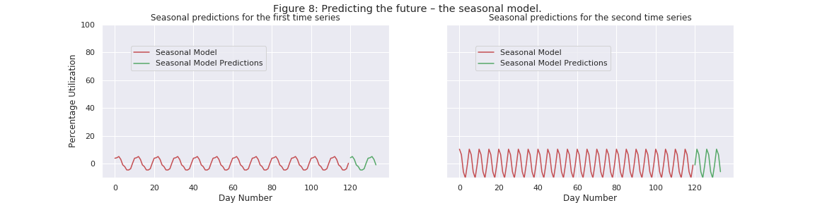
We have covered the steps to train the machine learning model to recognize trends. Now we can get to the exciting part - using our trained model to predict the future utilization. To do so, we must first understand the mechanics behind machine learning models. In a nutshell, any model is simply a mathematical function which accepts some kind of data as input and then produces estimates as output. In our case, the input is simply the sequence of day numbers (1, 2, 3, ..., 120) and the expected output is the value of the time series on that day. A good machine learning model is one that produces outputs which closely mirror the reality (the actual value of the time series that we have with us). Furthermore, in order to predict the future, we simply need to feed future day numbers (121, 122, ...) into our machine learning model and it will provide us approximate estimates regarding the future values of the time series. Finally, since our machine learning model is made up of two pieces, a seasonal component and a trend component, its prediction of the future will simply be the sum of these two components.
Predictions from the Seasonal Model
Since our seasonal model is merely a periodic and repetitive pattern, the future predictions are repetitions of the same pattern. We plot these repetitions for both time series in Figure 8.
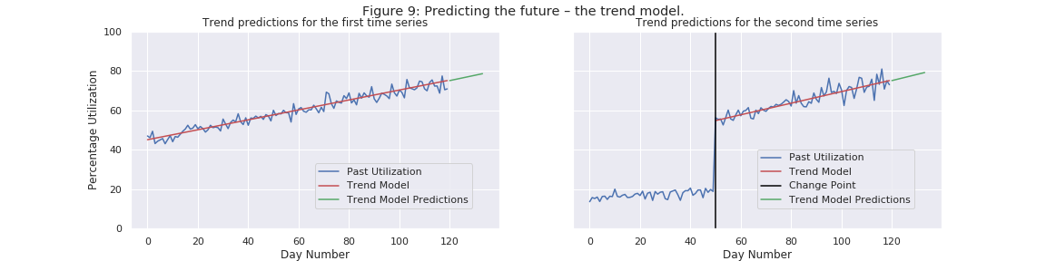
Predictions from the Trend Model
Similarly, given the mathematical model for our trend model, we can then use it to make predictions into the future. Those predictions are charted in Figure 9.
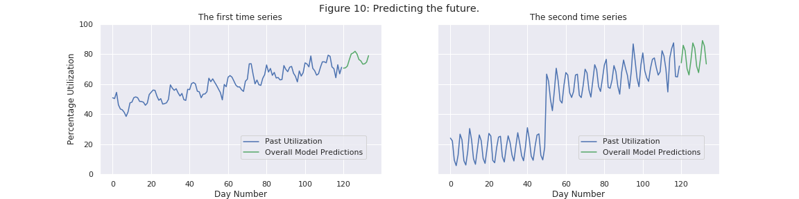
Overall Model Predictions
By summing up the predictions from the above two components, we obtain our overall model predictions. These are shown in Figure 10.
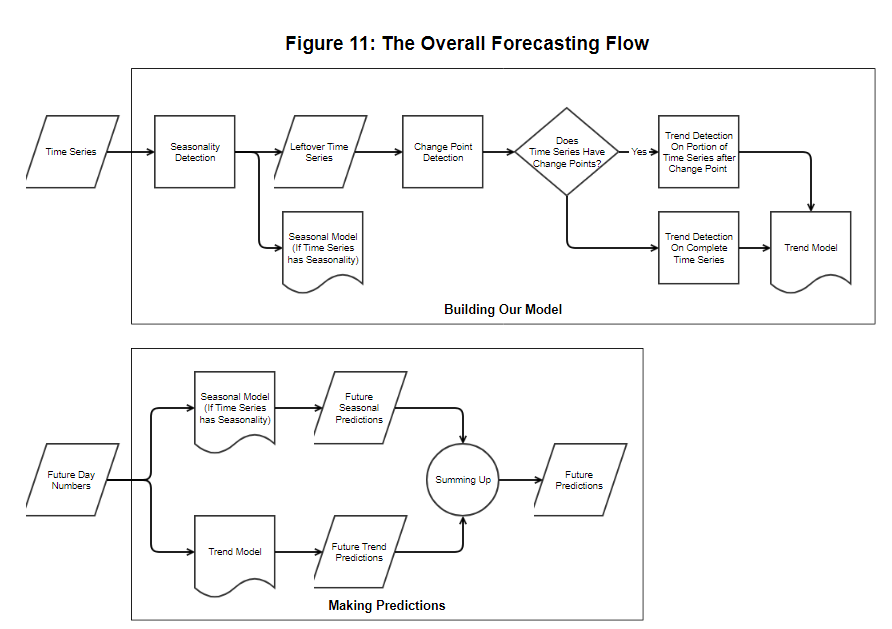
The Entire Model Flow
Below, the entire flow is summarized.
The Anomaly Detection Problem Statement
As we discussed earlier, meticulous capacity planning can help in preventing resource crunches most of the time, but sometimes the application behavior can spike or fall suddenly and unpredictably, and such cases are strong indicators of potential application failures. Suppose that the available capacity of a network link or a database drops suddenly and drastically due to a surge or a spike in usage. This kind of behavior can have significant impact on applications, and hence it is critical to notify the right people as quickly as possible. This is broadly termed as anomaly detection, and in order to explain it we shall consider the following problem statement:
If we have the past utilization data for a database, can we use it to identify whether the current utilization is anomalously high.
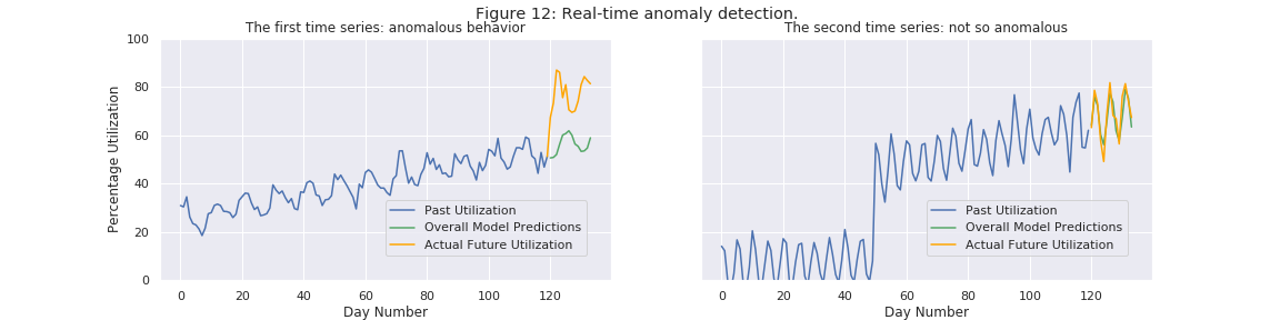
The approach that we take to tackle such a problem statement is to compare our forecasts with the current utilization. Given that our time series forecasting model provides a good estimate of the usual behavior of the time series, if the current utilization deviates significantly from the forecasted utilization then we can claim that this large deviation is an anomaly which might need human attention. In order to understand this better, let us consider the earlier case of the two time series.
Suppose that the actual future utilization turned out to be the orange line at the end in Figure 12 - in the first case, the orange line is way off from the predicted utilization while in the second, it is pretty close to it. We can say that the behavior of the first time series is anomalous and it might require human attention, but the second time series most likely does not. Our prediction model successfully predicted utilization in the second case, and adjusted resources so that no human attention is required. In the first case, our model can flag for human attention.
Conclusion
The machine learning system which we discussed in this post underpins an extensively used platform that simplifies capacity planning and can perform effective time series anomaly detection.
Going forward, we are:
- Working to open source our library for broader use.
- Continuously focusing on enhancing our machine learning models.
Credits
This model has been built and refined through the contributions of a number of team members including Madhavan Mukundan, Milan Someswar, Ankesh Jha, Nishu Kumari, Divyanshu Sharma, and Girija Vasireddy. Thank you also to Sayantan Sarkar, Anurag Ved, Krishnamurthy Vaidyanathan, and Bob Naccarella for the constant support and guidance.
Explore Opportunities at Goldman Sachs
We're hiring for several exciting roles. Visit our careers page to learn more.
See https://www.gs.com/disclaimer/global_email for important risk disclosures, conflicts of interest, and other terms and conditions relating to this blog and your reliance on information contained in it.
Solutions
Curated Data Security MasterData AnalyticsPlotTool ProPortfolio AnalyticsGS QuantTransaction BankingGS DAP®Liquidity Investing¹ Real-time data can be impacted by planned system maintenance, connectivity or availability issues stemming from related third-party service providers, or other intermittent or unplanned technology issues.
Transaction Banking services are offered by Goldman Sachs Bank USA ("GS Bank") and its affiliates. GS Bank is a New York State chartered bank, a member of the Federal Reserve System and a Member FDIC. For additional information, please see Bank Regulatory Information.
² Source: Goldman Sachs Asset Management, as of March 31, 2025.
Mosaic is a service mark of Goldman Sachs & Co. LLC. This service is made available in the United States by Goldman Sachs & Co. LLC and outside of the United States by Goldman Sachs International, or its local affiliates in accordance with applicable law and regulations. Goldman Sachs International and Goldman Sachs & Co. LLC are the distributors of the Goldman Sachs Funds. Depending upon the jurisdiction in which you are located, transactions in non-Goldman Sachs money market funds are affected by either Goldman Sachs & Co. LLC, a member of FINRA, SIPC and NYSE, or Goldman Sachs International. For additional information contact your Goldman Sachs representative. Goldman Sachs & Co. LLC, Goldman Sachs International, Goldman Sachs Liquidity Solutions, Goldman Sachs Asset Management, L.P., and the Goldman Sachs funds available through Goldman Sachs Liquidity Solutions and other affiliated entities, are under the common control of the Goldman Sachs Group, Inc.
Goldman Sachs & Co. LLC is a registered U.S. broker-dealer and futures commission merchant, and is subject to regulatory capital requirements including those imposed by the SEC, the U.S. Commodity Futures Trading Commission (CFTC), the Chicago Mercantile Exchange, the Financial Industry Regulatory Authority, Inc. and the National Futures Association.
FOR INSTITUTIONAL USE ONLY - NOT FOR USE AND/OR DISTRIBUTION TO RETAIL AND THE GENERAL PUBLIC.
This material is for informational purposes only. It is not an offer or solicitation to buy or sell any securities.
THIS MATERIAL DOES NOT CONSTITUTE AN OFFER OR SOLICITATION IN ANY JURISDICTION WHERE OR TO ANY PERSON TO WHOM IT WOULD BE UNAUTHORIZED OR UNLAWFUL TO DO SO. Prospective investors should inform themselves as to any applicable legal requirements and taxation and exchange control regulations in the countries of their citizenship, residence or domicile which might be relevant. This material is provided for informational purposes only and should not be construed as investment advice or an offer or solicitation to buy or sell securities. This material is not intended to be used as a general guide to investing, or as a source of any specific investment recommendations, and makes no implied or express recommendations concerning the manner in which any client's account should or would be handled, as appropriate investment strategies depend upon the client's investment objectives.
United Kingdom: In the United Kingdom, this material is a financial promotion and has been approved by Goldman Sachs Asset Management International, which is authorized and regulated in the United Kingdom by the Financial Conduct Authority.
European Economic Area (EEA): This marketing communication is disseminated by Goldman Sachs Asset Management B.V., including through its branches ("GSAM BV"). GSAM BV is authorised and regulated by the Dutch Authority for the Financial Markets (Autoriteit Financiële Markten, Vijzelgracht 50, 1017 HS Amsterdam, The Netherlands) as an alternative investment fund manager ("AIFM") as well as a manager of undertakings for collective investment in transferable securities ("UCITS"). Under its licence as an AIFM, the Manager is authorized to provide the investment services of (i) reception and transmission of orders in financial instruments; (ii) portfolio management; and (iii) investment advice. Under its licence as a manager of UCITS, the Manager is authorized to provide the investment services of (i) portfolio management; and (ii) investment advice.
Information about investor rights and collective redress mechanisms are available on www.gsam.com/responsible-investing (section Policies & Governance). Capital is at risk. Any claims arising out of or in connection with the terms and conditions of this disclaimer are governed by Dutch law.
To the extent it relates to custody activities, this financial promotion is disseminated by Goldman Sachs Bank Europe SE ("GSBE"), including through its authorised branches. GSBE is a credit institution incorporated in Germany and, within the Single Supervisory Mechanism established between those Member States of the European Union whose official currency is the Euro, subject to direct prudential supervision by the European Central Bank (Sonnemannstrasse 20, 60314 Frankfurt am Main, Germany) and in other respects supervised by German Federal Financial Supervisory Authority (Bundesanstalt für Finanzdienstleistungsaufsicht, BaFin) (Graurheindorfer Straße 108, 53117 Bonn, Germany; website: www.bafin.de) and Deutsche Bundesbank (Hauptverwaltung Frankfurt, Taunusanlage 5, 60329 Frankfurt am Main, Germany).
Switzerland: For Qualified Investor use only - Not for distribution to general public. This is marketing material. This document is provided to you by Goldman Sachs Bank AG, Zürich. Any future contractual relationships will be entered into with affiliates of Goldman Sachs Bank AG, which are domiciled outside of Switzerland. We would like to remind you that foreign (Non-Swiss) legal and regulatory systems may not provide the same level of protection in relation to client confidentiality and data protection as offered to you by Swiss law.
Asia excluding Japan: Please note that neither Goldman Sachs Asset Management (Hong Kong) Limited ("GSAMHK") or Goldman Sachs Asset Management (Singapore) Pte. Ltd. (Company Number: 201329851H ) ("GSAMS") nor any other entities involved in the Goldman Sachs Asset Management business that provide this material and information maintain any licenses, authorizations or registrations in Asia (other than Japan), except that it conducts businesses (subject to applicable local regulations) in and from the following jurisdictions: Hong Kong, Singapore, India and China. This material has been issued for use in or from Hong Kong by Goldman Sachs Asset Management (Hong Kong) Limited and in or from Singapore by Goldman Sachs Asset Management (Singapore) Pte. Ltd. (Company Number: 201329851H).
Australia: This material is distributed by Goldman Sachs Asset Management Australia Pty Ltd ABN 41 006 099 681, AFSL 228948 (‘GSAMA’) and is intended for viewing only by wholesale clients for the purposes of section 761G of the Corporations Act 2001 (Cth). This document may not be distributed to retail clients in Australia (as that term is defined in the Corporations Act 2001 (Cth)) or to the general public. This document may not be reproduced or distributed to any person without the prior consent of GSAMA. To the extent that this document contains any statement which may be considered to be financial product advice in Australia under the Corporations Act 2001 (Cth), that advice is intended to be given to the intended recipient of this document only, being a wholesale client for the purposes of the Corporations Act 2001 (Cth). Any advice provided in this document is provided by either of the following entities. They are exempt from the requirement to hold an Australian financial services licence under the Corporations Act of Australia and therefore do not hold any Australian Financial Services Licences, and are regulated under their respective laws applicable to their jurisdictions, which differ from Australian laws. Any financial services given to any person by these entities by distributing this document in Australia are provided to such persons pursuant to the respective ASIC Class Orders and ASIC Instrument mentioned below.
- Goldman Sachs Asset Management, LP (GSAMLP), Goldman Sachs & Co. LLC (GSCo), pursuant ASIC Class Order 03/1100; regulated by the US Securities and Exchange Commission under US laws.
- Goldman Sachs Asset Management International (GSAMI), Goldman Sachs International (GSI), pursuant to ASIC Class Order 03/1099; regulated by the Financial Conduct Authority; GSI is also authorized by the Prudential Regulation Authority, and both entities are under UK laws.
- Goldman Sachs Asset Management (Singapore) Pte. Ltd. (GSAMS), pursuant to ASIC Class Order 03/1102; regulated by the Monetary Authority of Singapore under Singaporean laws
- Goldman Sachs Asset Management (Hong Kong) Limited (GSAMHK), pursuant to ASIC Class Order 03/1103 and Goldman Sachs (Asia) LLC (GSALLC), pursuant to ASIC Instrument 04/0250; regulated by the Securities and Futures Commission of Hong Kong under Hong Kong laws
No offer to acquire any interest in a fund or a financial product is being made to you in this document. If the interests or financial products do become available in the future, the offer may be arranged by GSAMA in accordance with section 911A(2)(b) of the Corporations Act. GSAMA holds Australian Financial Services Licence No. 228948. Any offer will only be made in circumstances where disclosure is not required under Part 6D.2 of the Corporations Act or a product disclosure statement is not required to be given under Part 7.9 of the Corporations Act (as relevant).
FOR DISTRIBUTION ONLY TO FINANCIAL INSTITUTIONS, FINANCIAL SERVICES LICENSEES AND THEIR ADVISERS. NOT FOR VIEWING BY RETAIL CLIENTS OR MEMBERS OF THE GENERAL PUBLIC
Canada: This presentation has been communicated in Canada by GSAM LP, which is registered as a portfolio manager under securities legislation in all provinces of Canada and as a commodity trading manager under the commodity futures legislation of Ontario and as a derivatives adviser under the derivatives legislation of Quebec. GSAM LP is not registered to provide investment advisory or portfolio management services in respect of exchange-traded futures or options contracts in Manitoba and is not offering to provide such investment advisory or portfolio management services in Manitoba by delivery of this material.
Japan: This material has been issued or approved in Japan for the use of professional investors defined in Article 2 paragraph (31) of the Financial Instruments and Exchange Law ("FIEL"). Also, any description regarding investment strategies on or funds as collective investment scheme under Article 2 paragraph (2) item 5 or item 6 of FIEL has been approved only for Qualified Institutional Investors defined in Article 10 of Cabinet Office Ordinance of Definitions under Article 2 of FIEL.
Interest Rate Benchmark Transition Risks: This transaction may require payments or calculations to be made by reference to a benchmark rate ("Benchmark"), which will likely soon stop being published and be replaced by an alternative rate, or will be subject to substantial reform. These changes could have unpredictable and material consequences to the value, price, cost and/or performance of this transaction in the future and create material economic mismatches if you are using this transaction for hedging or similar purposes. Goldman Sachs may also have rights to exercise discretion to determine a replacement rate for the Benchmark for this transaction, including any price or other adjustments to account for differences between the replacement rate and the Benchmark, and the replacement rate and any adjustments we select may be inconsistent with, or contrary to, your interests or positions. Other material risks related to Benchmark reform can be found at https://www.gs.com/interest-rate-benchmark-transition-notice. Goldman Sachs cannot provide any assurances as to the materialization, consequences, or likely costs or expenses associated with any of the changes or risks arising from Benchmark reform, though they may be material. You are encouraged to seek independent legal, financial, tax, accounting, regulatory, or other appropriate advice on how changes to the Benchmark could impact this transaction.
Confidentiality: No part of this material may, without GSAM's prior written consent, be (i) copied, photocopied or duplicated in any form, by any means, or (ii) distributed to any person that is not an employee, officer, director, or authorized agent of the recipient.
GSAM Services Private Limited (formerly Goldman Sachs Asset Management (India) Private Limited) acts as the Investment Advisor, providing non-binding non-discretionary investment advice to dedicated offshore mandates, involving Indian and overseas securities, managed by GSAM entities based outside India. Members of the India team do not participate in the investment decision making process.