Introduction
Goldman Sachs runs on financial data and we, at Core Data Platform, provide services to manage data and optimize millions of data flows across all business segments.
Challenge
One such important data flow is Over the Counter (OTC) derivative contracts resulting from trades booked internally. These contracts are long, semi-structured and highly polymorphic.
Semi-structured means a long JSON file, about 30-40 levels deep, filled with dictionaries and arrays (even arrays of dictionaries and dictionary of arrays). Polymorphic means, there exist keys like ‘rate’ of the contract which can hold different forms like list, dictionary, or string based on the type of financial contract.
Given the dynamic nature of these contracts, the queries needed on these contracts are fast-moving. Our key data challenge here is to query the data quickly for keys at level 30 or more on an ad-hoc basis, without having to flatten this complex json data by data transformation processes which take days to write, are prone to errors and hard to maintain because the transformations needed are too many and keep on growing. This data (its shape, volume, and structure) is unique to finance, and it has been difficult to describe our problem to external data vendors without giving them access to real production data. And of course, providing such access is not possible as this data is private to the entities involved in the contract and thus quite sensitive.
Solution
Enter synthetic data generator!
We have created a synthetic data generator which produces anonymized data with the same statistical, polymorphic, and structural properties as production contractual data, while also preserving the primary key/foreign key relationships across datasets. While synthetic data generation tools are already prevalent in the industry, our data generator is specialized in capturing the unique data challenge that we have at Goldman Sachs in terms of the shape and volume of the data to be stored and the type of queries expected to run within X time based on the business expectation.
Deep dive
This blog post will deep dive into the novel statistical approach we took for implementation of synthetic data generator. Let us start with one production sample(left) and one synthetic sample (right) from synthetic data generator as shown below:
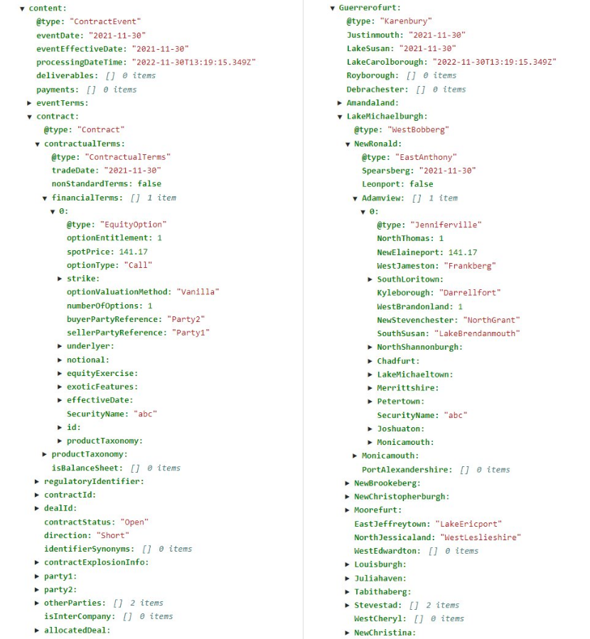
Understanding the complexity
Notice @type key of financialTerms(Adamview) in the left (right) sample? That’s the key representing the polymorphic part and deciding which other keys and data types will exist within financialTerms. financialTerms (Adamview) could be of multiple @types. In this case, it’s EquityOption (Jenniferville). As the type is EquityOption (Jenniferville), optionValuationMethod (Kyleborough) key exists and is of type String. If the type were ReturnSwap (Emilyfurt) instead, optionValuationMethod perhaps doesn’t exist (or Kyleborough could have been an array of dates). Basically, the jsons change structure and have many forms! And the structure can change at any nested level too.
The fundamental reason for modelling these jsons this way is that these contracts are very complex. So, we try to reuse the common structures that are modeled and shared across different types of contracts, and as such we end up with nesting and polymorphism, which we believe is still better than modeling every possible contract, as the possibilities of shape and combination are basically unlimited.
Let’s look at the algorithm we built for synthetic data generator. We start by taking a snapshot of production data and scanning it to capture the different “paths” and the probability distributions of each path and their value distributions.
Pseudo-algo for the synthetic data generator
- Create distribution files from reading production data.
- Distribution of exploded JSON path built with novel path system.
- Distribution of values of each path.
- Join Key distributions across datasets.
- Anonymize the distribution file.
- Generate new samples based on the distribution files.
.png)
Implementation
Let’s understand each of the steps in detail.
1. Create distribution files from reading production data
1a. Keys of the distribution file: Novel Path System
We scan through each sample and initialize a path from the root field of JSON. We keep on appending to that JSON path until fields with basic data types like String, Integer, Enum, Boolean, Date are encountered. Each field also has an optional [@type] and <Datatype> where @type is the key as shown in the sample above and Datatype is list, dict, String, Integer etc. One path will look like below:
[@typename1]FieldName1<DataType1>. [@typename2]FieldName2<DataType2>...
The intuition behind choosing the above path system is that every new [@typename] results in new sub paths due to polymorphic nature of the data. And that <datatype> dictates what kind of distribution to keep, for example if a list is seen, we capture the number of items in the list across data samples.
Example of a path is below (also shown in the diagram above) where we start from content and end at optionValuationMethod which is of String datatype storing relevant distributions on the way.
Examples of original paths each followed by their equivalent anonymized path:
content<dict>.[ContractEvent]contract<dict>.[Contract]financialTerms<list>.[EquityOption]optionValuationMethod<String>
Guerrerofurt<dict>.[Karenbury]LakeMichaelburgh<dict>.[WestBobberg]Adamview<list>.[Jenniferville]Kyleborough<String>
content<dict>.[ContractEvent]contract<dict>.[Contract]financialTerms<list>
Guerrerofurt<dict>.[Karenbury]LakeMichaelburgh<dict>.[WestBobberg]Adamview<list>
content<dict>.[ContractEvent]contract<dict>.[Contract]financialTerms<list>.[EquityOption]optionEntitlement<Integer
Guerrerofurt<dict>.[Karenbury]LakeMichaelburgh<dict>.[WestBobberg]Adamview<list>.[Jenniferville]NorthThomas<Integer>
To give an idea of scale, there were ~25k paths for the financial data snapshot that we worked with.
1b. Values of the distribution file:
(i) Distribution of basic datatypes:
For the fields with basic type, while reading the original data, we maintain following distributions:
- Float/Integer/Decimal/Number: Precision, sum, count, min, max and if_negative is stored. if_negative is a boolean which is 0 if all the values encountered for that field are positive, else 1. After all the samples are read, they are later aggregated into avg and std deviation (using the range rule of thumb).
- String: Max Length of the string is stored. Strings are considered Enums if number of unique values/total values seen < 0.2
- Enums: Weights of each enum values are stored. Weighted distribution is sampled.
- Boolean: Weights of each True, False is stored. Weighted distribution is sampled.
- Date/StrictDate/DateTime: Days from Jan 1, 1970, are stored. For datetime, hour values are ignored.
(ii) Distribution of lists/dictionaries:
For lists, the weighted frequency of the list size and distribution of every element is also saved as in (i). For dictionaries, each key distribution is saved as in (i)
(iii) Distribution of types:
For each <@typename>, the weighted frequency of each value is maintained to know how many samples to create of that path. Example:
{Adamview<dict>: {“Karenbury”: 98, “Emilyfurt”: 2}}
{financialTerms<dict>:{“EquityOption”: 50, “ReturnSwap”: 40, ...}}
2. Anonymize the distribution file:
Now, after the distribution file is created for the original data, to preserve the privacy of the original data, we anonymize the original distribution file. For this, we use faker class of python for unique city names. For every term in the distribution file, we replace the original term with the fake term to generate the fake distribution file. An inverted index is also maintained.
3. Generate new samples based on the distribution files.
After creating the anonymized distribution file, we traverse through each path and using the distributions, we generate the samples. Let us see how we generated each value for the basic datatypes:
- Strings: We already have the max length encountered. We randomly generate a string of that length.
- For Integers/Numbers and Dates: Given the average and standard deviation, a number is returned according to the normal distribution. For dates, that number is converted to a date, and for datetime a random hour is generated
- Others: For others, weighted frequency is used to generate the values.
PK/FK relationships across datasets:
Other than the complexity within one type of JSON, we have multiple datasets – each consisting of the JSON structure as discussed above and connected via (Primary Key, Foreign Key) relationships. Putting this in a business context - take the example of a contract leading to multiple deals. Contract Id will be shared across multiple deal ids. This is an example of 1:N relationship. We also have datasets with M:1 and M:N relationship similarly.
To solve this problem of generating multiple synthetic datasets with shared common keys, an important observation was that the business flow is directed - one contract results in multiple deals across regions and finally one aggregated payment across all of them – meaning there is no business loop (most of the times).
.PNG)
For calculating ‘N’, we scan the data to calculate the weighted frequency of join key and save as foreign-key-distributions having choices and weights as keys. Here, the choices reflect the number of samples of dataset B which are linked with one key of dataset A and weights are their weighted frequency. For instance,
{B : “foreign_distributions”:{“choices”:[1,2],”weights”:[3,4]} will indicate that one sample of A has created 1 sample of B with weighted frequency 3 and one sample of A has created 2 samples of B with weighted frequency 4.
For calculating ‘M’, we calculate the weighted frequency and save them as back-foreign-key-distributions having choices and weights as keys. Here, the choices reflect the number of samples of A which are linked to one key of B and weights are their weighted frequency. For instance,
{A : “back_foreign_distributions”:{“choices”:[1,2],”weights”:[3,4]} will indicate that one sample of B has created 1 sample of A with weighted frequency 3 and one sample of B has created 2 samples of A with weighted frequency 4.
How do we sample from these distributions?
We maintain the directed graph of business flow in a json.
“Contract”: {
“next”: "Deal",
“foreign_distributions”: {"choices": [1,2], "weights":[3,4]
"back_foreign_distributions: "",
"back": ""
}
The process starts with creating X samples of root table – in above example Contract table. For each sample of contract table created, we sample from foreign distributions to create N samples of next table, in this case deal table. If back foreign distributions exist, we create M-1 samples of previous table.
Easy to use Python toolkit
Our synthetic data generator is a python toolkit available for quick installation via pip. It takes in the number of samples as a parameter. Here number of samples means the number of root samples (read number of json objects) in the directed graph (ref section: PK/FK Relationships across datasets). For each root sample, the rest of the connected datasets with their weighed PK/FK distributions get automatically created in different folders. The python application uses multiprocessing and spawns as many processes as number of cores available. Each process generates an independent sample (and N or M samples of other related datasets based on relationships). So, the application can scale very easily with the number of cores provided. We can provide either one big box or multiple small boxes.
Anonymized queries
While getting the shape and structure of synthetic data was important, equally important and challenging was to get a set of representative queries which we could share with vendors and set the right performance expectations on.
Our approach was to connect with engineers who create the complex data transformation processes today on the contractual data, understand their business use case and work with them to come up with a set of representative queries of different complexity. Example of queries: Simple at query, Unpacking JSON based on attribute value, Complex joins across multiple datasets including self joins
A simple unpacking of json example would look like below where there are multiple case statements for fetching unadjusted date across different contract types like Return Swap or Equity Forward or Equity Option:
case when v:CONTENT:contract:contractualTerms:financialTerms[0]:"@type"::String = 'ReturnSwap'
then v:CONTENT:contract:contractualTerms:financialTerms[0]:returnSwapLeg[0]:valuation:finalValuationDate:unadjustedDate
when v:CONTENT:contract:contractualTerms:financialTerms[0]:"@type"::String = 'EquityForward'
then v:CONTENT:contract:contractualTerms:financialTerms[0]:equityExercise:equityEuropeanExercise:expirationDate:adjustableDate:unadjustedDate
when v:CONTENT:contract:contractualTerms:financialTerms[0]:"@type"::String = 'EquityOption' and v:CONTENT:contract.contractualTerms.financialTerms[0].productTaxonomy.secdbTradableClassification::String in ('Eq B','Eq O')
then v:CONTENT:contract:contractualTerms:financialTerms[0]:equityExercise.equityEuropeanExercise.expirationDate.adjustableDate.unadjustedDate
To share with vendors outside, we anonymized the queries with the anonymized index we created while scanning the data and shared with users. The anonymized query for above snippet looks like:
case when v:Guerrerofurt:LakeMichaelburgh:NewRonald:Adamview[0]:"@type"::String = 'Emilyfurt'
then v:Guerrerofurt:LakeMichaelburgh:NewRonald:Adamview[0]:NorthGregoryside[0]:PortDavidburgh:SouthAlexander:EastMegan
when v:Guerrerofurt:LakeMichaelburgh:NewRonald:Adamview[0]:"@type"::String = 'EastAllison'
then v:Guerrerofurt:LakeMichaelburgh:NewRonald:Adamview[0]:LakeMichaeltown:SouthVincentland:Lindaview:SouthKimberlyview:EastMegan
when v:Guerrerofurt:LakeMichaelburgh:NewRonald:Adamview[0]:"@type"::String = 'Jenniferville' and v:Guerrerofurt:LakeMichaelburgh.NewRonald.Adamview[0].Monicamouth.EastBryanberg::String in ('00787CookMewsApt910','8236AlvarezLanding','7387ArthurFieldsSuite294')
then v:Guerrerofurt:LakeMichaelburgh:NewRonald:Adamview[0]:LakeMichaeltown.SouthTimothyside.Lindaview.SouthKimberlyview.EastMegan
Our initial expectation from vendors is to run the tool for a few million samples, run anonymized queries on them and share their performance. We ask vendors to scale further based on initial evaluation.
Summary
The synthetic data approach has been valuable for us to benchmark vendors and in bringing clarity, transparency and visibility to finance data challenges both inside and outside the firm. We are looking forward to sharing more data engineering problems with the whole industry. Cheers!
Credits
This model was built and refined through the contributions of several team members including Pragya Srivastava, Abner Espinoza and Rahul Thakur. Thank you also to Dimitris Tsementzis, Toh Ne Win, Ajeya Kumar, Gisha Babby, Ramanathan Narayanan, Regina Chan, Pierre De Belen, Neema Raphael and Stefano Stefani for their constant support and guidance.
See https://www.gs.com/disclaimer/global_email for important risk disclosures, conflicts of interest, and other terms and conditions relating to this blog and your reliance on information contained in it.
Solutions
Curated Data Security MasterData AnalyticsPlotTool ProPortfolio AnalyticsGS QuantTransaction BankingGS DAP®Liquidity Investing¹ Real-time data can be impacted by planned system maintenance, connectivity or availability issues stemming from related third-party service providers, or other intermittent or unplanned technology issues.
Transaction Banking services are offered by Goldman Sachs Bank USA ("GS Bank") and its affiliates. GS Bank is a New York State chartered bank, a member of the Federal Reserve System and a Member FDIC. For additional information, please see Bank Regulatory Information.
² Source: Goldman Sachs Asset Management, as of March 31, 2025.
Mosaic is a service mark of Goldman Sachs & Co. LLC. This service is made available in the United States by Goldman Sachs & Co. LLC and outside of the United States by Goldman Sachs International, or its local affiliates in accordance with applicable law and regulations. Goldman Sachs International and Goldman Sachs & Co. LLC are the distributors of the Goldman Sachs Funds. Depending upon the jurisdiction in which you are located, transactions in non-Goldman Sachs money market funds are affected by either Goldman Sachs & Co. LLC, a member of FINRA, SIPC and NYSE, or Goldman Sachs International. For additional information contact your Goldman Sachs representative. Goldman Sachs & Co. LLC, Goldman Sachs International, Goldman Sachs Liquidity Solutions, Goldman Sachs Asset Management, L.P., and the Goldman Sachs funds available through Goldman Sachs Liquidity Solutions and other affiliated entities, are under the common control of the Goldman Sachs Group, Inc.
Goldman Sachs & Co. LLC is a registered U.S. broker-dealer and futures commission merchant, and is subject to regulatory capital requirements including those imposed by the SEC, the U.S. Commodity Futures Trading Commission (CFTC), the Chicago Mercantile Exchange, the Financial Industry Regulatory Authority, Inc. and the National Futures Association.
FOR INSTITUTIONAL USE ONLY - NOT FOR USE AND/OR DISTRIBUTION TO RETAIL AND THE GENERAL PUBLIC.
This material is for informational purposes only. It is not an offer or solicitation to buy or sell any securities.
THIS MATERIAL DOES NOT CONSTITUTE AN OFFER OR SOLICITATION IN ANY JURISDICTION WHERE OR TO ANY PERSON TO WHOM IT WOULD BE UNAUTHORIZED OR UNLAWFUL TO DO SO. Prospective investors should inform themselves as to any applicable legal requirements and taxation and exchange control regulations in the countries of their citizenship, residence or domicile which might be relevant. This material is provided for informational purposes only and should not be construed as investment advice or an offer or solicitation to buy or sell securities. This material is not intended to be used as a general guide to investing, or as a source of any specific investment recommendations, and makes no implied or express recommendations concerning the manner in which any client's account should or would be handled, as appropriate investment strategies depend upon the client's investment objectives.
United Kingdom: In the United Kingdom, this material is a financial promotion and has been approved by Goldman Sachs Asset Management International, which is authorized and regulated in the United Kingdom by the Financial Conduct Authority.
European Economic Area (EEA): This marketing communication is disseminated by Goldman Sachs Asset Management B.V., including through its branches ("GSAM BV"). GSAM BV is authorised and regulated by the Dutch Authority for the Financial Markets (Autoriteit Financiële Markten, Vijzelgracht 50, 1017 HS Amsterdam, The Netherlands) as an alternative investment fund manager ("AIFM") as well as a manager of undertakings for collective investment in transferable securities ("UCITS"). Under its licence as an AIFM, the Manager is authorized to provide the investment services of (i) reception and transmission of orders in financial instruments; (ii) portfolio management; and (iii) investment advice. Under its licence as a manager of UCITS, the Manager is authorized to provide the investment services of (i) portfolio management; and (ii) investment advice.
Information about investor rights and collective redress mechanisms are available on www.gsam.com/responsible-investing (section Policies & Governance). Capital is at risk. Any claims arising out of or in connection with the terms and conditions of this disclaimer are governed by Dutch law.
To the extent it relates to custody activities, this financial promotion is disseminated by Goldman Sachs Bank Europe SE ("GSBE"), including through its authorised branches. GSBE is a credit institution incorporated in Germany and, within the Single Supervisory Mechanism established between those Member States of the European Union whose official currency is the Euro, subject to direct prudential supervision by the European Central Bank (Sonnemannstrasse 20, 60314 Frankfurt am Main, Germany) and in other respects supervised by German Federal Financial Supervisory Authority (Bundesanstalt für Finanzdienstleistungsaufsicht, BaFin) (Graurheindorfer Straße 108, 53117 Bonn, Germany; website: www.bafin.de) and Deutsche Bundesbank (Hauptverwaltung Frankfurt, Taunusanlage 5, 60329 Frankfurt am Main, Germany).
Switzerland: For Qualified Investor use only - Not for distribution to general public. This is marketing material. This document is provided to you by Goldman Sachs Bank AG, Zürich. Any future contractual relationships will be entered into with affiliates of Goldman Sachs Bank AG, which are domiciled outside of Switzerland. We would like to remind you that foreign (Non-Swiss) legal and regulatory systems may not provide the same level of protection in relation to client confidentiality and data protection as offered to you by Swiss law.
Asia excluding Japan: Please note that neither Goldman Sachs Asset Management (Hong Kong) Limited ("GSAMHK") or Goldman Sachs Asset Management (Singapore) Pte. Ltd. (Company Number: 201329851H ) ("GSAMS") nor any other entities involved in the Goldman Sachs Asset Management business that provide this material and information maintain any licenses, authorizations or registrations in Asia (other than Japan), except that it conducts businesses (subject to applicable local regulations) in and from the following jurisdictions: Hong Kong, Singapore, India and China. This material has been issued for use in or from Hong Kong by Goldman Sachs Asset Management (Hong Kong) Limited and in or from Singapore by Goldman Sachs Asset Management (Singapore) Pte. Ltd. (Company Number: 201329851H).
Australia: This material is distributed by Goldman Sachs Asset Management Australia Pty Ltd ABN 41 006 099 681, AFSL 228948 (‘GSAMA’) and is intended for viewing only by wholesale clients for the purposes of section 761G of the Corporations Act 2001 (Cth). This document may not be distributed to retail clients in Australia (as that term is defined in the Corporations Act 2001 (Cth)) or to the general public. This document may not be reproduced or distributed to any person without the prior consent of GSAMA. To the extent that this document contains any statement which may be considered to be financial product advice in Australia under the Corporations Act 2001 (Cth), that advice is intended to be given to the intended recipient of this document only, being a wholesale client for the purposes of the Corporations Act 2001 (Cth). Any advice provided in this document is provided by either of the following entities. They are exempt from the requirement to hold an Australian financial services licence under the Corporations Act of Australia and therefore do not hold any Australian Financial Services Licences, and are regulated under their respective laws applicable to their jurisdictions, which differ from Australian laws. Any financial services given to any person by these entities by distributing this document in Australia are provided to such persons pursuant to the respective ASIC Class Orders and ASIC Instrument mentioned below.
- Goldman Sachs Asset Management, LP (GSAMLP), Goldman Sachs & Co. LLC (GSCo), pursuant ASIC Class Order 03/1100; regulated by the US Securities and Exchange Commission under US laws.
- Goldman Sachs Asset Management International (GSAMI), Goldman Sachs International (GSI), pursuant to ASIC Class Order 03/1099; regulated by the Financial Conduct Authority; GSI is also authorized by the Prudential Regulation Authority, and both entities are under UK laws.
- Goldman Sachs Asset Management (Singapore) Pte. Ltd. (GSAMS), pursuant to ASIC Class Order 03/1102; regulated by the Monetary Authority of Singapore under Singaporean laws
- Goldman Sachs Asset Management (Hong Kong) Limited (GSAMHK), pursuant to ASIC Class Order 03/1103 and Goldman Sachs (Asia) LLC (GSALLC), pursuant to ASIC Instrument 04/0250; regulated by the Securities and Futures Commission of Hong Kong under Hong Kong laws
No offer to acquire any interest in a fund or a financial product is being made to you in this document. If the interests or financial products do become available in the future, the offer may be arranged by GSAMA in accordance with section 911A(2)(b) of the Corporations Act. GSAMA holds Australian Financial Services Licence No. 228948. Any offer will only be made in circumstances where disclosure is not required under Part 6D.2 of the Corporations Act or a product disclosure statement is not required to be given under Part 7.9 of the Corporations Act (as relevant).
FOR DISTRIBUTION ONLY TO FINANCIAL INSTITUTIONS, FINANCIAL SERVICES LICENSEES AND THEIR ADVISERS. NOT FOR VIEWING BY RETAIL CLIENTS OR MEMBERS OF THE GENERAL PUBLIC
Canada: This presentation has been communicated in Canada by GSAM LP, which is registered as a portfolio manager under securities legislation in all provinces of Canada and as a commodity trading manager under the commodity futures legislation of Ontario and as a derivatives adviser under the derivatives legislation of Quebec. GSAM LP is not registered to provide investment advisory or portfolio management services in respect of exchange-traded futures or options contracts in Manitoba and is not offering to provide such investment advisory or portfolio management services in Manitoba by delivery of this material.
Japan: This material has been issued or approved in Japan for the use of professional investors defined in Article 2 paragraph (31) of the Financial Instruments and Exchange Law ("FIEL"). Also, any description regarding investment strategies on or funds as collective investment scheme under Article 2 paragraph (2) item 5 or item 6 of FIEL has been approved only for Qualified Institutional Investors defined in Article 10 of Cabinet Office Ordinance of Definitions under Article 2 of FIEL.
Interest Rate Benchmark Transition Risks: This transaction may require payments or calculations to be made by reference to a benchmark rate ("Benchmark"), which will likely soon stop being published and be replaced by an alternative rate, or will be subject to substantial reform. These changes could have unpredictable and material consequences to the value, price, cost and/or performance of this transaction in the future and create material economic mismatches if you are using this transaction for hedging or similar purposes. Goldman Sachs may also have rights to exercise discretion to determine a replacement rate for the Benchmark for this transaction, including any price or other adjustments to account for differences between the replacement rate and the Benchmark, and the replacement rate and any adjustments we select may be inconsistent with, or contrary to, your interests or positions. Other material risks related to Benchmark reform can be found at https://www.gs.com/interest-rate-benchmark-transition-notice. Goldman Sachs cannot provide any assurances as to the materialization, consequences, or likely costs or expenses associated with any of the changes or risks arising from Benchmark reform, though they may be material. You are encouraged to seek independent legal, financial, tax, accounting, regulatory, or other appropriate advice on how changes to the Benchmark could impact this transaction.
Confidentiality: No part of this material may, without GSAM's prior written consent, be (i) copied, photocopied or duplicated in any form, by any means, or (ii) distributed to any person that is not an employee, officer, director, or authorized agent of the recipient.
GSAM Services Private Limited (formerly Goldman Sachs Asset Management (India) Private Limited) acts as the Investment Advisor, providing non-binding non-discretionary investment advice to dedicated offshore mandates, involving Indian and overseas securities, managed by GSAM entities based outside India. Members of the India team do not participate in the investment decision making process.