Hedging using Machine Learning Techniques

As systematic and macro factors dominate the investment landscape, we see equity investors move away from one-size-fits all hedging strategies to more precise ways to separate intended and unintended risks and isolate alpha.

If you are a fundamental equity investor, take concentrated positions in single names, or have significant idiosyncratic risk that is otherwise difficult to hedge, this highly customizable correlation-based approach is for you. Traditional factor-based hedges can fare poorly when most of the risk cannot be explained by factors – in those instances this approach can allow for much better correlation to offset risk as well as a number of ways to guide which names get included while ensuring a high level of tradability by controlling liquidity and borrow costs.

In this notebook, we will showcase how to leverage this approach through one of our most popular tools, the Marquee Performance Hedger.

Additionally, based on feedback we have received from top users, we are adding the ability to easily run and compare hedges in Python through GS Quant as well as new modeling techniques, two of whose key advantages are:

• Increased accuracy through reduced overfitting
• More control by allowing the user to specify how concentrated or diversified the hedge portfolio is

Let's get started with GS Quant

To begin, read the GS Quant Getting Started guide

Start every session with authenticating with your unique client id and secret. If you don't have a registered app, create one here. read_product_data scope is required for the functionality covered in this example.

from gs_quant.session import GsSession, Environment
GsSession.use(client_id=None, client_secret=None, scopes=('read_product_data',))

Define Your Positions to Hedge and Your Hedge Universe

The hedger takes in the initial portfolio as a PositionSet object. You can define your positions as a list of identifiers with quantities or alternatively, as a list of identifiers with weights, along with a reference notional value. The date corresponds to the hedge date.

In addition, you need to define your universe of candidates for hedge constituents as a list of identifiers.

GS Quant will resolve all identifiers (Bloomberg IDs, SEDOLs, RICs, etc) historically as of the hedge date

import datetime as dt
from gs_quant.markets.position_set import Position, PositionSe

positions = PositionSet(
        date=dt.date(day=24, month=9, year=2021),
        positions=[
            Position(identifier='AAPL UW', quantity=26),
            Position(identifier='GS UN', quantity=51)
        ]
    )

positions.resolve()

universe = ['SPX']

Define Your Hedge Exclusions

The HedgeExclusions class offers a clean way to specify any assets, countries, regions, sectors, and/or industries you would like to exclude from your hedge. Each attribute takes in a list of strings. In this example, let's try excluding Goldman Sachs and all assets in Mexico, Europe, the Utilities sector, the Airlines industry.

from gs_quant.markets.hedge import HedgeExclusions

exclusions = HedgeExclusions(assets=['GS UN'],
                             countries=['Mexico'],
                             regions=['Europe'],
                             sectors=['Utilities'],
                             industries=['Airlines'])

Define Your Hedge Constraints

Rather than excluding an industry or region entirely, you can also constrain how much each makes up in your hedge, and you can do so by leveraging the HedgeConstraints class. Each attribute takes in a list of Constraint objects, each of which has a name attribute, along with minimum and maximum that should be expressed as positive numbers between 0 and 100.

In addition to constraining assets, countries, regions, sectors, and industries, it's also possible to constrain your hedge to only include assets that have an ESG score between a specified range. All data is pulled as of your hedge date from the GIR SUSTAIN ESG Headline Metrics Dataset. For more information on the various ESG metrics available, please visit the dataset page here.

In this example, let's constrain our hedge to only include at most 20% Software assets by weight. In addition, let's request a hedge with only assets that have a G Headline Percentile Score of above 75%.

from gs_quant.markets.hedge import HedgeConstraints, Constraint,

constraints = HedgeConstraints(sectors=[Constraint(constraint_name='Software', minimum=0, maximum=20)],
                               esg=[Constraint(constraint_name='gPercentile', minimum=75, maximum=100)])

Define Any Other Parameters

The PerformanceHedgeParameters wraps all the performance hedge parameters, including the positions, exclusions, and constraints, into an object to be passed into a PerformanceHedge. Along with the parameters defined above, the following optional parameters can also be passed in:

from gs_quant.markets.hedge import PerformanceHedgeParameters

parameters = PerformanceHedgeParameters(
    initial_portfolio=positions,
    universe=universe,
    exclusions=exclusions,
    constraints=constraints
)

Calculate Your Hedge

It's finally time to run the parameters into the Marquee Hedger. Once defined, a PerformanceHedge can be calculated in just one line.

from gs_quant.markets.hedge import PerformanceHedge

hedge = PerformanceHedge(parameters)
all_results = hedge.calculate()

Pull Hedge Results

That's it! Once calculated, you can pull the results right from the PerformanceHedge object.

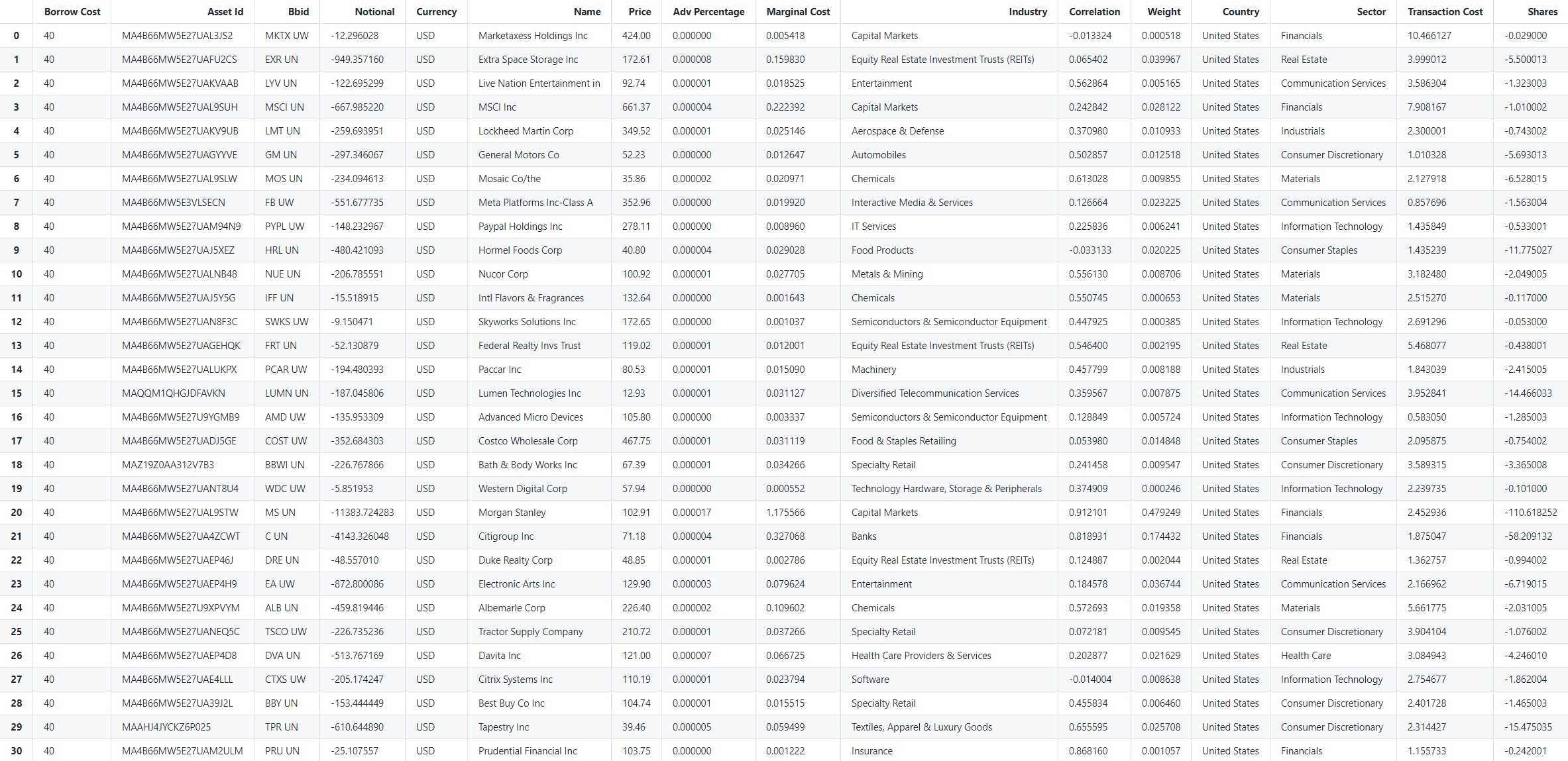
Constituents

Let's pull the constituents metadata of the resulting hedge:

from IPython.display import display

hedge_constituents = hedge.get_constituents()
display(hedge_constituents)

Output:

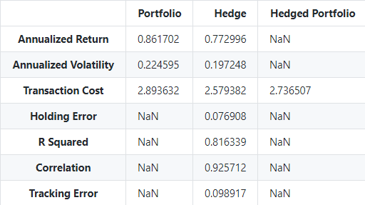
Stats

Next let's pull a table of general stats like transaction cost, annualized volatility, annualized return, and more:

stats = hedge.get_statistics()
display(stats)

Output:

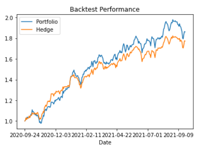
Backtest Performance

It's also possible to pull a timeseries of the performance of both the initial portfolio and the hedge for the observation period:

backtest_performance = hedge.get_backtest_performance()

backtest_performance.plot(title='Backtest Performance')

Output:

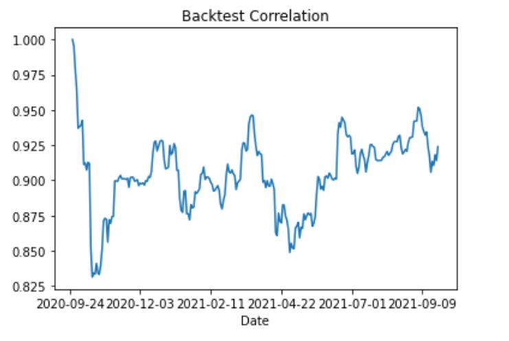
Backtest Correlation

It's also possible to pull a timeseries of the correlation between the hedge and portfolio for the observation period by leveraging GS Quant econometric function correlation:

from gs_quant.timeseries.helper import Window
from gs_quant.timeseries.econometrics import correlation

backtest_correlation = correlation(backtest_performance['Portfolio'], backtest_performance['Hedge'], Window(44, 0))
backtest_correlation.plot(title='Backtest Correlation')

Output:

Create a new Portfolio or Basket

If you would like to turn your hedge into a basket or a portfolio, you can convert it into a PositionSet object and pass it into a new portfolio or basket.

positions = []
for index, row in hedge_constituents.iterrows():
    positions.append(Position(identifier=row['Bbid'], asset_id=row['Asset Id'], quantity=row['Shares']))

position_set = PositionSet(date=business_day_offset(dt.date.today(), -1, roll='forward'),
                           positions=positions)

Portfolio

Learn more about creating portfolios [here].

from gs_quant.markets.portfolio import Portfolio
from gs_quant.markets.portfolio_manager import PortfolioManager

new_portfolio = Portfolio(name="Hedge as Portfolio")
new_portfolio.save()

pm = PortfolioManager(new_portfolio.id)
pm.update_positions([position_set])

Basket

Learn more about creating baskets here.

from gs_quant.markets.baskets import Basket
from gs_quant.markets.indices_utils import ReturnType

my_basket = Basket()

my_basket.name = 'My New Custom Basket'
my_basket.ticker = 'GSMBXXXX'
my_basket.currency = 'USD'
my_basket.publish_to_reuters = True

my_basket.return_type = ReturnType.PRICE_RETURN

my_basket.position_set = position_set
my_basket.create()

You're all set; Congrats!

Other questions? Reach out to the Portfolio Analytics team!